The Racing Line

It's easy to take a picture of a track and draw a reasonable racing line. You approach the turns on the outside and take a smooth line that cuts across to the inside and then back to the outside. If there are several turns close together, you have to compromise, making a line that would not be ideal for any one turn in isolation. But even for complicated sections, it's easy to freehand a decent racing line. But how can we describe this process precisely enough to allow a computer to calculate the racing line?

Figure 1: A simple example track. The total length of the centerline is 1133m.

As an example, take a look at the track in figure 1. If you were trying to set a fast lap time, you would stick to the right-hand side of the road down the long straight and make a smooth curve through the first two left turns. You would cross the track to set up for the right-hand turn 3. This turn is followed closely by the sharp left-hand turn 4, so you can't take the ideal line through both; you need to compromise the exit of 3 to make a decent entrance to 4. After that you sweep through 5 and set up to make the widest possible curve through turn 6 so that you carry as much speed as possible down the long straight.

From this exercise it seems that a good racing line is one that minimizes curvature. We can find a path that minimizes curvature by simulating a chain of masses on spring-loaded hinges that loops around the track and connects to itself. We will start by placing the masses on the centerline of the track and constrain them to stay on the track surface. As we propagate the system forward in time, the springs will open the hinges and the masses will shift until we approach a smooth curve that minimizes the energy stored in the springs.

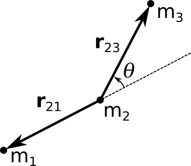
Figure 2: Three nodes on the calculated racing line. The angular displacement $\theta$ produces a restoring torque.

The force acting on a given mass $m_2$ can be calculated from the relative positions of its neighbors as shown in figure 2. Let's start by assuming that closing the hinge produces a torque proportional to the angular displacement.

$$\mathbf{N}_2 = \ensuremath{\mathbf{r}_{\mathrm{23}}} \times \mathbf{F}_3 = -k \theta \ensuremath{\hat{\mathbf{n}}}$$ (1)

where is the vector from $m_2$ to $m_3$ and is the unit vector in the direction of $\ensuremath{\mathbf{r}_{\mathrm{23}}} \times \ensuremath{\mathbf{r}_{\mathrm{21}}}$. The force on $m_3$ is then

$$\mathbf{F}_3 = -\frac{k}{\vert\ensuremath{\mathbf{r}_{\math... ...n}}} \times \ensuremath{\ensuremath{\hat{\mathbf{r}}}_{23}})$$ (2)

We can calculate $\theta \ensuremath{\hat{\mathbf{n}}}$ from the cross product of and .

$$\ensuremath{\mathbf{r}_{\mathrm{23}}} \times \ensuremath{\mathbf{r}_{\mathrm{21}}} = \vert\ensuremath{\mathbf{r}_{\mathrm{23}}}\vert\vert\ensuremath{\mathbf{r}_{\mathrm{21}}}\vert \sin (\pi - \theta) \ensuremath{\hat{\mathbf{n}}}$$ (3)

$$= \vert\ensuremath{\mathbf{r}_{\mathrm{23}}}\vert\vert\ensuremath{\mathbf{r}_{\mathrm{21}}}\vert \sin \theta \ensuremath{\hat{\mathbf{n}}}$$ (4)

$$\sin \theta \ensuremath{\hat{\mathbf{n}}} = \ensuremath{\mathbf{r}_{\mathrm{23}}} \times \ensuremath{\mathbf{... ...h{\mathbf{r}_{\mathrm{23}}}\vert\vert\ensuremath{\mathbf{r}_{\mathrm{21}}}\vert$$ (5)

$$= \ensuremath{\ensuremath{\hat{\mathbf{r}}}_{23}} \times \ensuremath{\ensuremath{\hat{\mathbf{r}}}_{21}}$$ (6)

Since we're trying to model a smooth curve, we expect the bend at each node to be small so that we can use $x$ for $\sin x$. If these conditions are not met then the number of nodes is insufficient to model a smooth curve and should be increased.

$$\theta \ensuremath{\hat{\mathbf{n}}} = \ensuremath{\ensurem... ...{23}} \times \ensuremath{\ensuremath{\hat{\mathbf{r}}}_{21}}$$ (7)

Substituting into equation 2 we get

$$\mathbf{F}_3 = \frac{k}{\vert\ensuremath{\mathbf{r}_{\mathr... ...21}}) \times \ensuremath{\ensuremath{\hat{\mathbf{r}}}_{23}}$$ (8)

By symmetry, we find that $\mathbf{F}_1 = \mathbf{F}_3$ and $\mathbf{F}_2 = -2\mathbf{F}_3$ provided that $\theta$ is small.

We can define the curvature vector $\mathbf{c}$ at $m_3$ to be

$$\mathbf{c} = \ensuremath{\hat{\mathbf{n}}}/R = \theta \ensu... ...\mathbf{n}}} / \vert\ensuremath{\mathbf{r}_{\mathrm{23}}}\vert$$ (9)

where $R$ is the radius of curvature of the racing line at $m_3$. The angle $\theta$ is the angle between $m_2$ and $m_3$ from the center of curvature. If $m_1$, $m_2$, and $m_3$ are equally spaced along a circular arc then this is the same as the angular displacement defined above. We expect these conditions to hold if the nodes are sufficiently close together. We can rewrite equation 8 as

$$\mathbf{F}_3 = -k \mathbf{c} \times \ensuremath{\ensuremath{\hat{\mathbf{r}}}_{23}}$$ (10)

We will use the magnitude of the curvature vector to determine the maximum speed for computer-controlled cars at a given point on the track.

The forces are calculated for each contiguous triplet of nodes. The total force on a given node is the sum of the forces exerted by its neighbor's hinges, and the reaction forces from the force of its own hinge on its neighbors. Instead of allowing the nodes to move freely in all directions, we constrain the nodes to move across the track. This constraint improves stability which allows us to use higher hinge torques which in turn gives faster convergence. The node's motion is damped to improve stability.

Once the total force on each node is calculated a new position for the node is calculated using Newton's laws of motion and the Euler method.

$$\ensuremath{\mathbf{v}_{\mathrm{i+1}}} = \ensuremath{\mathbf{v}_{\mathrm{i}}} + (\mathbf{F}/m - c \ensuremath{\mathbf{v}_{\mathrm{i}}}) \Delta t$$ (11)

$$\ensuremath{\mathbf{r}_{\mathrm{i+1}}} = \ensuremath{\mathbf{r}_{\mathrm{i}}} + \ensuremath{\mathbf{v}_{\mathrm{i+1}}} \Delta t$$ (12)

After many iterations the positions should stabilize. The racing line can be a bit distorted at very sharp turns because the nodes become close together as they move to the apex. Deleting every other node after convergence helps to smooth it out.

The curvature need not be calculated until propagation is finished, but equation 10 shows that it may be convenient to calculate curvature as the forces are calculated during propagation.

Figure 3: A calculated racing line for the example track. A line of 139 nodes was propagated for 800 iterations. The stiffness was 1.0Nm/rad and the damping coefficient was 0.1kg/s. The time step and mass were set to unity. The nodes are shown as red dots. Cyan tinting indicates the degree of left-hand curvature, magenta indicates right-hard curvature.

The racing line calculated for the example track shown in figure 3 matches well with what we would expect. However, there is still a little distortion around the sharp turn 4. The curve flattens out a bit after the apex.